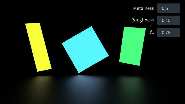
A new Magnum example implements an analytic method for area light shading presented in the paper “Real-Time Polygonal-Light Shading with Linearly Transformed Cosines”, by Eric Heitz, Jonathan Dupuy, Stephen Hill and David Neubelt.
The code is available through the Area Lights example page in the documentation and the example has also a live web version linked below. This blog post explains the basics of shading with linearly transformed cosines (LTCs) and how Magnum was used for the implementation.
Shading with LTCs
To understand linearly transformed cosines I will start off by explaining some basics. If you already know what BRDFs are, you may want to skip the next paragraph or two.
Binary Reflectance Distribution Functions
When shading a point on a surface, physically, you need to take all incoming rays from every direction into account. Some light rays affect the final color of the shaded point more than others — depending on their direction, the view direction and the properties of the material.
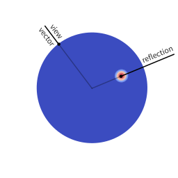
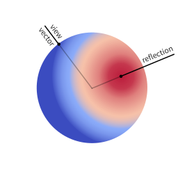
A perfect mirror, for example, may take only the exact reflection of the view vector into account, as can be seen in figure (a), whereas a more diffuse material will be affected by all or most incoming rays similarly or equally, as visualized in figure (b).
These figures show spherical distributions: imagine you want to shade a point on a surface (the point where the view vector is reflected). Imagine a ray of light hitting this point, it will pierce through the colored sphere at some location. The color at that location on the sphere indicates how much this ray will affect the color of the surface point: the more red, the higher the effect.
The function that describes how much effect an incoming light ray has for given viewing and incoming light angles, is called BRDF. This function is very specific to every material. As this is very impractical for real-time rendering and art pipelines, it is common to instead use a so called parametric BRDF; a function which is able to approximate many different BRDFs of different materials using intuitive parameters, e.g. roughness or metalness.
There are many parametric BRDFs out there: the GGX microfacet BRDF, the Schlick BRDF and the Cook-Torrance BRDF. I recomment playing around with them in Disney’s BRDF Explorer.
Shading area lights
With point lights, shading is really simple as you only have a single incoming ray — assuming you do not want to take indirect rays into account. You can get the appropriate factor (of how much of that ray will be reflected in view direction) from the BRDF using the view angle and light angle, multiply that with the light intensity and that is already it.
With area lights, it is a lot more complicated, as you have an infinite amount of incoming rays. The final intensity of the shaded point is the integral over the BRDF in the domain of the polygon of the light (which, projected onto the spherical distribution, is a spherical polygon).
This is a problem, because we do not have an analytical solution to integrating over arbitrary spherical distributions. Instead, such a solution is known only for very specific distributions, the uniform sphere or the cosine distribution for example.
So, how can we still do it without radically approximating the area light?
Linearly transformed cosines
The genius of the paper is that the authors realized they can transform spherical distributions using linear transforms (scaling, rotation and skewing) and that this leaves the value of the integral unchanged.


Image source: Eric Heitz’s Research Page
You can therefore transform a spherical distribution to look like another spherical distribution. This means that you can transform something like the cosine distribution to look like a specific BRDF given a certain view angle. You can then — because the integral is unaffected by the linear transform — integrate over the cosine distribution, to which an analytical solution is known, instead of integrating over the BRDF.
As this BRDF is view dependent, you need a transformation for every incident
view angle, and every parameter of a parametric BRDF. In the paper, they achieve
this by fitting a 3x3 matrix (for the transformation) for a set of sampled values
for the BRDF parameter alpha (roughness) of the GGX Microfacet BRDF as well as
the viewing angle.
The 3x3 matrices have only four really significant components. Consequently they can be stored in an RGBA texture.
For shading we need the inverse matrices to transform the polygon of the light. Originally it is of course in the space of the BRDF over which we do not know how to integrate over. If we apply the inverse matrix to polygon, it is then in the space of the cosine distribution over which we can integrate instead.
Image source: Eric Heitz’s Research Page
Implementation
To aid my understanding of the method, I implemented a basic version of LTC shading using Magnum. The C++ example provided with the paper uses the Schlick BRDF and already contained textures with the fitted inverse LTC matrices.
The code of the Magnum example is well documented and if you are interested, I recommend you go check it out. Instead of giving a thorough line by line explanation, I will point out some of the features in Magnum that were most helpful to me. They are more generally applicable to other projects as well.
Loading LTC matrix textures
The original C++ implementation provided with the paper already contained .dds files for the fitted inverse LTC matrices. Many thanks to Eric Heitz, who was kind enough to let me use these for the Magnum example.
I packed these dds files as a resource into the binary (makes porting to web
easier later). It was a matter of simply adding the resources.conf, telling
Corrade to compile it in your CMakeLists.txt…
corrade_add_resource(AreaLights_RESOURCES resources.conf)

add_executable(magnum-arealights AreaLightsExample.cpp ${AreaLights_RESOURCES})
… and then loading the texture from the resource memory using DdsImporter:
/* Load the DdsImporter plugin */
PluginManager::Manager<Trade::AbstractImporter> manager;
Containers::Pointer<Trade::AbstractImporter> importer =
    manager.loadAndInstantiate("DdsImporter");
if(!importer) std::exit(1);

/* Get the resource containing the images */
const Utility::Resource rs{"arealights-data"};
if(!importer->openData(rs.getRaw("ltc_mat.dds")))
    std::exit(2);

/* Set texture data and parameters */
Containers::Optional<Trade::ImageData2D> image = importer->image2D(0);
CORRADE_INTERNAL_ASSERT(image);
_ltcMat.setWrapping(SamplerWrapping::ClampToEdge)
    .setMagnificationFilter(SamplerFilter::Linear)
    .setMinificationFilter(SamplerFilter::Linear)
    .setStorage(1, GL::TextureFormat::RGBA32F, image->size())
    .setSubImage(0, {}, *image);

/* Bind the texture for use in the shader */
_shader.bindLtcMatTexture(_ltcMat);
Shader Hot-Reload
During shader development, you will not want to restart your application every time you make a change to the GLSL shader code. It is rather nice to be able to just hit F5 and see the changes immediately instead.
It turns out that if you implemented an GL::AbstractShaderProgram, hot-reloading is just a matter of reinstantiating it:
/* Reload the shader */
_shader = AreaLightShader{};
Yes, it is that simple.
Often you will compile your shader files as resources in Magnum (as done in the example). To use shaders from a resource in your GL::AbstractShaderProgram you would again make use of Utility::Resource:
GL::Shader vert{version, GL::Shader::Type::Vertex};
GL::Shader frag{version, GL::Shader::Type::Fragment};

/* Load shaders from compiled-in resource */
Utility::Resource rs("arealights-data");
vert.addSource(rs.get("AreaLights.vert"));
frag.addSource(rs.get("AreaLights.frag"));
In this case you will need to override the resource group using Utility::Resource::overrideGroup() to load the resource from the original file rather than from memory before hot-reloading:
/* Reload the shader */
Utility::Resource::overrideGroup("arealights-data", "<path>/resources.conf");
_shader = Shaders::AreaLight{};
Thanks
Final appreciations go to Eric Heitz, Jonathan Dupuy, Stephen Hill and David Neubelt for publishing a incredibly well written paper with a ton of supplemental material and effort around it — and of course Magnum for making it viable to quickly get this basic implementation running.
Thank you for reading! I’ll be back.
About the author
Jonathan Hale lives for Virtual Reality. Developer and project manager at Vhite Rabbit. Follow him on Twitter: @Squareys

Guest Posts
This is a guest post by an external author. Do you also have something interesting to say? A success story worth sharing? We’ll be happy to publish it. See the introductory post for details.